metadynminer3d

	News
1	Introduction
2	Source
3	Usage
3.1	Installation
3.2	Reading HILLS files
3.3	Calculation of free energy surface
3.4	Plotting of free energy surface
3.5	Identification of minima
3.6	Calculation of free energy profiles
3.7	Removing one collective variable
3.8	Nudged Elastic Band
4	Tips and tricks
5	References
6	Contact
7	Terms of use
8	Privacy

News

Metadynminer and Metadynminer3D paper out in R Journal:
D. Trapl, V. Spiwok: Analysis of the Results of Metadynamics Simulations by metadynminer and metadynminer3d. R Journal 14(3) 46-58 (2022).

Videos from Metadynminer Plumed Masterclass (February 2022) are available at Youtube (thanks to Plumed!!!):

Video from Metadynminer webinar (31 May 2019) is available at Youtube (thanks to ELIXIR Slovenia!!!):

metadynminer3d has been published.

Introduction

metadynminer3d is an addendum to the package metadynminer. metadynminer is R packages for reading, analysis and visualization of metadynamics HILLS files produced by Plumed[1]. metadynminer3d visualizes 3D free energy surfaces by rgl package. It reads HILLS files from Plumed, calculates free energy surfaces by fast Bias Sum algorithm [2] and finds minima.

Source

	https://github.com/spiwokv/metadynminer3d
	https://github.com/spiwokv/metadynminer3d/actions/
	https://ci.appveyor.com/project/spiwokv/metadynminer3d
	https://cran.r-project.org/package=metadynminer3d

	https://codecov.io/gh/spiwokv/metadynminer3d/

Usage

Instalation

To install R see http://www.metadynamics.cz/metadynminer/index.html#par3.1.

Install a stable version of metadynminer3d from CRAN by starting the R environment and typing:

> install.packages("metadynminer3d")

metadynminer is installed together with metadynminer3d, unless already installed.

If you want to install a development version of the package from github, you need to install devtools:

> install.packages("devtools")
> library(devtools)
> devtools::install_github("spiwokv/metadynminer3d")

Next, invoke metadynminer:

> library(metadynminer3d)
Loading required package: metadynminer
Loading required package: rgl

metadynminer is loaded together with metadynminer3d, unless already loaded.

Help can be obtained by the function help() with the name of the function as the argument, or by a question mark followed by the name of the function:

> help(read.hills3d)
> ?read.hills

Reading HILLS files

metadynminer3d is used in similar way to metadynminer. The main difference is in loading of hills file. This is done by function read.hills3d (see difference from read.hills in metadynminer). A Plumed HILLS file can be loaded by typing:

> hillsf<-read.hills3d("HILLS")
3D HILLS file read

This assumes that the hills file is in the working directory. If not you can specify the path (e.g. "../mymetadynamics/HILLS"). Alternatively you can check path by typing:

> getwd()
[1] "/home/yourlogin/somedirectory"

and you can change working directory by typing:

> setwd("/home/yourlogin/directory")

(may be useful in MS Windows). Hills file can be also loaded from a web site by using its URL:

> hillsf<-read.hills3d("http://www.metadynamics.cz/metadynminer/data/HILLS3d")
3D HILLS file read

metadynminer3d accepts only hills files with three collective variables (for one or two collective variables use metadynminer).

If some of collective variables is periodic (usually a torsion) it is necessary to specify this fact at the moment of loading of hills file by parameter per. It must be set to a vector with one or three logical elements for individual collective variables, respectively. In R, a vector can be created using function c() by specify its elements, e.g. per=c(TRUE, TRUE, TRUE) provided that all collective variables are periodic.

> hillsf<-read.hills3d("HILLS", per=c(TRUE, TRUE, TRUE))
3D HILLS file read

Collective variables are not periodic by default.

Period of a periodic collective variable is by default set to -π to +π. It can be changed by setting parameters pcv1, pcv2 and pcv3, for example

> hillsf<-read.hills3d("HILLS", per=c(TRUE, TRUE, TRUE), pcv1=c(0,2*pi))
3D HILLS file read

metadynminer3d contains a preloaded data set for Alanine Dipeptide in water with Ramachandran angles φ and ψ and angle ω as collective variables (called acealanme3d).

Metadynamics simulations are very often split into multiple runs with RESTART Plumed keyword. Hills file obtained from restarted simulations usually contain discontinuous values in the time column (i.e. they start from zero at every restart). This may complicate visualization. It is possible to solve this problem when loading hills by setting ignoretime=TRUE in the read.hills3d function. It will take the time of addition of the first hill and use multiplicates of this value for all other hills.

However, a user can load hills from restarted simulations without this option. First, wrong time values do not affect calculations of free energy surfaces. Second, the option ignoretime=TRUE can be used later for selected functions (see later).

The package metadynminer3d provides print and summary functions for its objects, including hills file. Try it by typing:

> acealanme3d
3D hills file HILLS2d with 30000 lines
> summary(acealanme3d)
3D hills file HILLS3d with 30000 lines
The CV1 ranges from -3.141557 to 3.141574
The CV2 ranges from -3.141248 to 3.141401
The CV3 ranges from -3.141561 to 3.141578

Hills file objects can be concatenated by addition (+) operation:

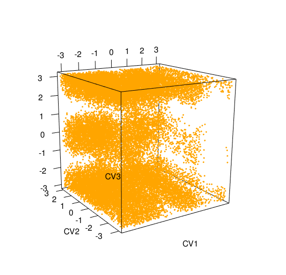
> acealanme3d+acealanme3d
3D hills file HILLS3d with 60000 lines

metadynminer3d provides plot function for its objects. Hills file with three collective variable will be pllotted as a 3D scatter plot of collective variable.

> plot(acealanme3d)

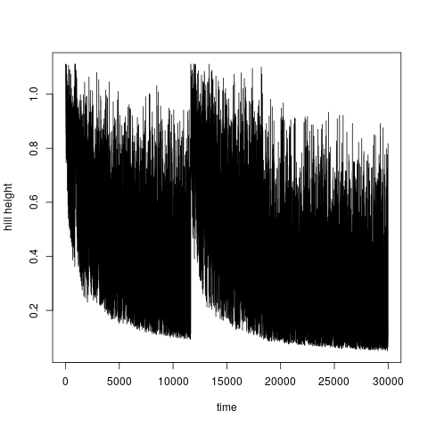
In a plot you can modify labels of axes (xlab, ylab and zlab), title (main) and subtitle (sub).

In well tempered metadynamics [3] it is useful to see evolution of heights of hills. This can be plotted by typing:

> plotheights(acealanme3d)

It is again possible to use ignoretime=TRUE for this function if you have not used this option in read.hills.

Calculation of free energy surface

Free energy surface is calculated by summing hills using function fes:

> tfes<-fes(hillsf)

Summing hills is much less expensive than a metadynamics simulation, nevertheless, it can be a slow process if number of hills exceeds 10,000. We developed a Bias Sum algorithm [2] to accelerate this calculation. Instead of evaluation exp(-||s-S_t||²/2σ²) for every hill it calculates a single Gaussian hill and relocates it. This function is not available for simulations with variable hill widths. As an alternative it is possible to calculate free energy surface by conventional way (function fes2). This function works with variable hill widths:

> tfes<-fes2(hillsf)

Hills can be summed for whole simulation (default) or for selected hills. The range can be controlled by imin and imax. These are indexes of first and last hill to be summed.

> tfes<-fes(hillsf, imin=5000, imax=10000)

By default the free energy surface is calculated for 64x64x64 grid points. This can be changed by npoints option.

Two free energy surfaces can be added and subtracted:

> tfes
3D free energy surface with 64 x 64 x 64 points, maximum -0.0005099049 and minimum -77.69544
> tfes+tfes
3D free energy surface with 256 x 256 points, maximum -0.00101981 and minimum -155.3909
> tfes-tfes
Warning: FES obtained by subtraction of two FESes
 will inherit hills only from the first FES
3D free energy surface with 64 x 64 x 64 points, maximum 0 and minimum 0

It is possible to add or subtract a constant. Free energy surface can be also multiplied or divided by a constant:

> tfes/4.184
Warning: division of FES will divide
 the FES but not hill heights
3D free energy surface with 64 x 64 x 64 points, maximum -0.0001218702 and minimum -18.56966

It is possible to calculate minimum and maximum of free energy surface by functions min and max, respectively. This can be used, for example, to convert a free energy surface so that the global minimum is equal to zero:

> tfes-min(tfes)
3D free energy surface with 64 x 64 x 64 points, maximum 77.69493 and minimum 0

The function summary function gives the same output as print for free energy surface object:

tfes
3D free energy surface with 64 x 64 x 64 points, maximum -0.0005099049 and minimum -77.69544
summary(tfes)
3D free energy surface with 64 x 64 x 64 points, maximum -0.0005099049 and minimum -77.69544

Plotting of free energy surface

Free energy surface can be plotted by function plot:

> tfes<-fes(acealanme3d)
> plot(tfes, level=-40)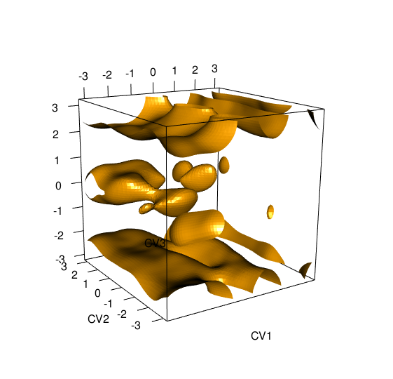

It is plotted as an isosurface at energy given by value level. It is possible to plot multiple isosurfaces by setting the parameter level to a vector (e.g. c(-40,-20)). It is possible to change color of isosurface by parameter col. It is also possible to change transparency of the isosurface by alpha. Parameters col and alpha can be used as vectors for vector input of level. It is possible to switch from solid to wireframe isosurface by setting fill=FALSE.

Identification of minima

Free energy minima corresponds to stable or metastable states of the studied system. You can use function fesminima to automatically locate free energy minima on the free energy surface:

> tfes<-fes(acealanme3d)
> minima<-fesminima(tfes)

This function divides the free energy surface into 8x8x8 equivalent bins. For each bin it finds its energy minimum. Next, it checks whether these minima are local minima of the whole surface. These minima are collected, sorted and labeled by alphabet letters. The number of bins can be modified by parameter nbins.

Functions print and summary are available for a minima object:

> minima
$minima

   letter CV1bin CV2bin CV3bin        CV1        CV2         CV3 free_energy
1       A     19     59     64 -1.3463969  2.6429272  3.14159265   -77.69544
2       B      7     60     64 -2.5431941  2.7426603  3.14159265   -77.01237
3       C     19     30      1 -1.3463969 -0.2493328 -3.14159265   -75.45002
4       D     42     37      1  0.9474645  0.4487990 -3.14159265   -72.31305
5       E     43     64      1  1.0471976  3.1415927 -3.14159265   -65.68216
6       F      5     60     33 -2.7426603  2.7426603  0.04986655   -61.81688
7       G     21     60     32 -1.1469307  2.7426603 -0.04986655   -61.53924
8       H     41     43     33  0.8477314  1.0471976  0.04986655   -52.84217
9       I      7     45     33 -2.5431941  1.2466638  0.04986655   -52.56641
10      J     20     26     31 -1.2466638 -0.6482652 -0.14959965   -50.88729
11      K     44     60     32  1.1469307  2.7426603 -0.04986655   -50.27426
12      L      6     25     31 -2.6429272 -0.7479983 -0.14959965   -40.22922
13      M     42     12     33  0.9474645 -2.0445286  0.04986655   -23.45578
> summary(minima)

   letter CV1bin CV2bin CV3bin        CV1        CV2         CV3 free_energy
1       A     19     59     64 -1.3463969  2.6429272  3.14159265   -77.69544
2       B      7     60     64 -2.5431941  2.7426603  3.14159265   -77.01237
3       C     19     30      1 -1.3463969 -0.2493328 -3.14159265   -75.45002
4       D     42     37      1  0.9474645  0.4487990 -3.14159265   -72.31305
5       E     43     64      1  1.0471976  3.1415927 -3.14159265   -65.68216
6       F      5     60     33 -2.7426603  2.7426603  0.04986655   -61.81688
7       G     21     60     32 -1.1469307  2.7426603 -0.04986655   -61.53924
8       H     41     43     33  0.8477314  1.0471976  0.04986655   -52.84217
9       I      7     45     33 -2.5431941  1.2466638  0.04986655   -52.56641
10      J     20     26     31 -1.2466638 -0.6482652 -0.14959965   -50.88729
11      K     44     60     32  1.1469307  2.7426603 -0.04986655   -50.27426
12      L      6     25     31 -2.6429272 -0.7479983 -0.14959965   -40.22922
13      M     42     12     33  0.9474645 -2.0445286  0.04986655   -23.45578
   relative_pop          pop
1  3.376498e+13 4.359308e+01
2  2.567614e+13 3.314979e+01
3  1.372429e+13 1.771908e+01
4  3.901889e+12 5.037628e+00
5  2.733340e+11 3.528944e-01
6  5.803151e+10 7.492297e-02
7  5.191820e+10 6.703024e-02
8  1.588441e+09 2.050795e-03
9  1.422182e+09 1.836142e-03
10 7.254113e+08 9.365597e-04
11 5.673389e+08 7.324765e-04
12 1.011072e+07 1.305368e-05
13 1.213841e+04 1.567159e-08

The function summary calculate equilibrium populations of each minimum in percent. Keep in mind that these values were calculated from free energies of minima points, not by integrating populations of each free energy minimum basin. These values are dependent on temperature and energy units. By default these are set to temp=300 and eunit="kJ/mol". The parameter eunit can be set to "kJ/mol" or "kcal/mol".

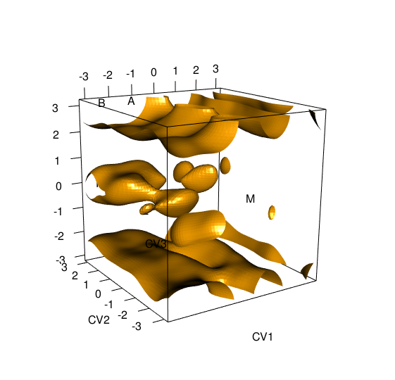
Sometimes it is useful to add some point in the space of collective variables to the list of automatically identified minima. This can be done by making a "fake" minimum and adding it to the list:

> minima<-fesminima(tfes)+oneminimum(tfes, cv1=0, cv2=0, cv3=0)
> minima

   letter CV1bin CV2bin CV3bin        CV1        CV2         CV3 free_energy
1       A     19     59     64 -1.3463969  2.6429272  3.14159265 -77.6954404
2       B      7     60     64 -2.5431941  2.7426603  3.14159265 -77.0123738
3       C     19     30      1 -1.3463969 -0.2493328 -3.14159265 -75.4500204
4       D     42     37      1  0.9474645  0.4487990 -3.14159265 -72.3130486
5       E     43     64      1  1.0471976  3.1415927 -3.14159265 -65.6821638
6       F      5     60     33 -2.7426603  2.7426603  0.04986655 -61.8168813
7       G     21     60     32 -1.1469307  2.7426603 -0.04986655 -61.5392350
8       H     41     43     33  0.8477314  1.0471976  0.04986655 -52.8421689
9       I      7     45     33 -2.5431941  1.2466638  0.04986655 -52.5664080
10      J     20     26     31 -1.2466638 -0.6482652 -0.14959965 -50.8872905
11      K     44     60     32  1.1469307  2.7426603 -0.04986655 -50.2742608
12      L      6     25     31 -2.6429272 -0.7479983 -0.14959965 -40.2292175
13      M     42     12     33  0.9474645 -2.0445286  0.04986655 -23.4557814
14      N     33     33     33  0.0000000  0.0000000  0.00000000  -0.5402724

This will create the same set of minima with the additional one placed in the point {0,0,0}.

The function plot applied on a minima object provides a same image as for the corresponding free energy energy minimum object with additional minima labels:

> plot(minima)

Calculation of free energy profiles

Convergence can be evaluated by function feprof:

> tfes<-fes(acealanme3d)
> minima<-fesminima(tfes)
> prof<-feprof(minima)

This function calculates evolution of free energy differences between each minimum and the global minimum (global at the end of simulation). Free energy of the global minimum is always zero.

Similarly to functions fes and fes2 it is possible to specify the range of hills by imax (imin option is not available because it does not make sense to calculate profiles from other point than from the start).

It is possible to use functions print and summary on free energy profile:

> prof

   letter CV1bin CV2bin CV3bin        CV1        CV2         CV3 free_energy
1       A     19     59     64 -1.3463969  2.6429272  3.14159265   -77.69544
2       B      7     60     64 -2.5431941  2.7426603  3.14159265   -77.01237
3       C     19     30      1 -1.3463969 -0.2493328 -3.14159265   -75.45002
4       D     42     37      1  0.9474645  0.4487990 -3.14159265   -72.31305
5       E     43     64      1  1.0471976  3.1415927 -3.14159265   -65.68216
6       F      5     60     33 -2.7426603  2.7426603  0.04986655   -61.81688
7       G     21     60     32 -1.1469307  2.7426603 -0.04986655   -61.53924
8       H     41     43     33  0.8477314  1.0471976  0.04986655   -52.84217
9       I      7     45     33 -2.5431941  1.2466638  0.04986655   -52.56641
10      J     20     26     31 -1.2466638 -0.6482652 -0.14959965   -50.88729
11      K     44     60     32  1.1469307  2.7426603 -0.04986655   -50.27426
12      L      6     25     31 -2.6429272 -0.7479983 -0.14959965   -40.22922
13      M     42     12     33  0.9474645 -2.0445286  0.04986655   -23.45578

Summary to be corrected!!!

The function summary prints minimal and maximal free energy difference for time range specified by imind and imaxd. For example, it is possible to calculate the free energy surface from all hills and evaluate convergence of the free energy difference in last 10,000 hills:

> tfes<-fes(acealanme)
> minima<-fesminima(tfes)
> prof<-feprof(minima)
> summary(prof, imind=20000, imaxd=30000)

Summary to be corrected!!!

Profiles can be plotted using plot function:

> plot(prof)

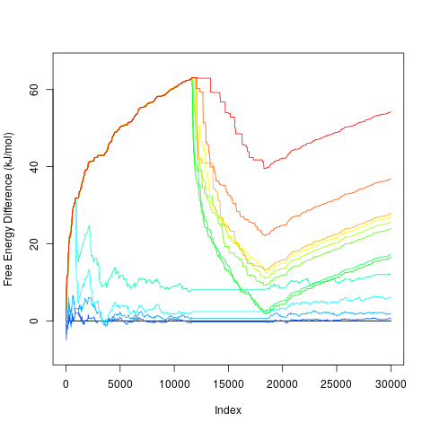
By default it plots profiles for all free energy minima. It is possible to specify minima to be plotted by which followed by the vector of indexes of minima.

Removing one collective variable

This option is not available in metadynminer3d.

Nudged Elastic Band

This option is not available in metadynminer3d.

Tips and Tricks

Publication quality figures

Following script can be used to generate a publication quality figure:

> tfes<-fes(acealanme3d)
> plot(tfes)

Change window size, zoom in and rotate if necessary, then (without closing the window) type:

> rgl.snapshot(filename="plot.png")

Publication of interactive FES on web

You can save free energy surface in WebGL and present it on a web site by typing:

> writeWebGL(filename="index.html")

Making movie

It is possible to make movie of rotation of the plot by:

> movie3d(spin3d(axis=c(0,0,1)), duration=3)

This will create a three-second animated GIF file of rotation around z-axis. It needs installation of convert command from ImageMagic program. Alternatively, the command:

> movie3d(spin3d(axis=c(0,0,1)), duration=3,
+         dir=".", convert=FALSE)

These files can be concatenated by a movie making program such as mencoder. For movie of flooding look at metadynminer.

Modifying aspect ratio of box

The aspect ratio of the box can be modified by:

> aspect3d(2, 1, 1)

after plot command. This makes the x-axis twice longer than other axes.

References

G.A. Tribello, M. Bonomi, D. Branduardi, C. Camilloni, G. Bussi: PLUMED2: New feathers for an old bird. Comput. Phys. Commun. 185, 604 (2014).
P. Hosek, V. Spiwok: Metadyn View: Fast web-based viewer of free energy surfaces calculated by metadynamics. Comput. Phys. Commun. 198, 222 (2016).
A. Barducci, G. Bussi, M. Parrinello: Well-tempered metadynamics: A smoothly converging and tunable free-energy method. Phys. Rev. Lett. 100, 020603 (2008).

Contact

Author + maintenance: Vojtech Spiwok (spiwokv<you-know-what>vscht.cz)

Contents